Introduction to Data Structures
Data Structure is a way of collecting and organising data in such a way that we can perform operations on these data in an effective way. Data Structures is about rendering data elements in terms of some relationship, for better organization and storage. For example, we have data player’s name “Virat” and age 26. Here “Virat” is of String data type and 26 is of integer data type.
We can organize this data as a record like Player record. Now we can collect and store player’s records in a file or database as a data structure. For example: “Dhoni” 30, “Gambhir” 31, “Sehwag” 33
In simple language, Data Structures are structures programmed to store ordered data, so that various operations can be performed on it easily.
Basic types of Data Structures
As we discussed above, anything that can store data can be called as a data strucure, hence Integer, Float, Boolean, Char etc, all are data structures. They are known as Primitive Data Structures.
Then we also have some complex Data Structures, which are used to store large and connected data. Some example of Abstract Data Structure are :
- Linked List
- Tree
- Graph
- Stack, Queue etc.
All these data structures allow us to perform different operations on data. We select these data structures based on which type of operation is required. We will look into these data structures in more details in our later lessons.

What is Algorithm ?
An algorithm is a finite set of instructions or logic, written in order, to accomplish a certain predefined task. Algorithm is not the complete code or program, it is just the core logic(solution) of a problem, which can be expressed either as an informal high level description as pseudocode or using a flowchart.
An algorithm is said to be efficient and fast, if it takes less time to execute and consumes less memory space. The performance of an algorithm is measured on the basis of following properties :
- Time Complexity
- Space Complexity
Space Complexity
Its the amount of memory space required by the algorithm, during the course of its execution. Space complexity must be taken seriously for multi-user systems and in situations where limited memory is available.
An algorithm generally requires space for following components :
- Instruction Space : Its the space required to store the executable version of the program. This space is fixed, but varies depending upon the number of lines of code in the program.
- Data Space : Its the space required to store all the constants and variables value.
- Environment Space : Its the space required to store the environment information needed to resume the suspended function.
Time Complexity
Time Complexity is a way to represent the amount of time needed by the program to run to completion. We will study this in details in our section.
NOTE: Before going deep into data structure, you should have a good knowledge of programming either in C or in C++ or Java.
Time Complexity of Algorithms
Time complexity of an algorithm signifies the total time required by the program to run to completion. The time complexity of algorithms is most commonly expressed using the big O notation.
Time Complexity is most commonly estimated by counting the number of elementary functions performed by the algorithm. And since the algorithm’s performance may vary with different types of input data, hence for an algorithm we usually use the worst-case Time complexity of an algorithm because that is the maximum time taken for any input size.
Calculating Time Complexity
Now lets tap onto the next big topic related to Time complexity, which is How to Calculate Time Complexity. It becomes very confusing some times, but we will try to explain it in the simplest way.
Now the most common metric for calculating time complexity is Big O notation. This removes all constant factors so that the running time can be estimated in relation to N, as N approaches infinity. In general you can think of it like this :
statement;
Above we have a single statement. Its Time Complexity will be Constant. The running time of the statement will not change in relation to N.
for(i=0; i < N; i++)
{
  statement;
}
The time complexity for the above algorithm will be Linear. The running time of the loop is directly proportional to N. When N doubles, so does the running time.
for(i=0; i < N; i++)
{
  for(j=0; j < N;j++)
  {
    statement;
  }
}
This time, the time complexity for the above code will be Quadratic. The running time of the two loops is proportional to the square of N. When N doubles, the running time increases by N * N.
while(low <= high)
{
  mid = (low + high) / 2;
  if (target < list[mid])
    high = mid - 1;
  else if (target > list[mid])
    low = mid + 1;
  else break;
}
This is an algorithm to break a set of numbers into halves, to search a particular field(we will study this in detail later). Now, this algorithm will have a Logarithmic Time Complexity. The running time of the algorithm is proportional to the number of times N can be divided by 2(N is high-low here). This is because the algorithm divides the working area in half with each iteration.
void quicksort(int list[], int left, int right)
{
  int pivot = partition(list, left, right);
  quicksort(list, left, pivot - 1);
  quicksort(list, pivot + 1, right);
}
Taking the previous algorithm forward, above we have a small logic of Quick Sort(we will study this in detail later). Now in Quick Sort, we divide the list into halves every time, but we repeat the iteration N times(where N is the size of list). Hence time complexity will be N*log( N ). The running time consists of N loops (iterative or recursive) that are logarithmic, thus the algorithm is a combination of linear and logarithmic.
NOTE : In general, doing something with every item in one dimension is linear, doing something with every item in two dimensions is quadratic, and dividing the working area in half is logarithmic.
Types of Notations for Time Complexity
Now we will discuss and understand the various notations used for Time Complexity.
- Big Oh denotes “fewer than or the same as” <expression> iterations.
- Big Omega denotes “more than or the same as” <expression> iterations.
- Big Theta denotes “the same as” <expression> iterations.
- Little Oh denotes “fewer than” <expression> iterations.
- Little Omega denotes “more than” <expression> iterations.
Understanding Notations of Time Complexity with Example
O(expression) is the set of functions that grow slower than or at the same rate as expression.
Omega(expression) is the set of functions that grow faster than or at the same rate as expression.
Theta(expression) consist of all the functions that lie in both O(expression) and Omega(expression).
Suppose you’ve calculated that an algorithm takes f(n) operations, where,
f(n) = 3*n^2 + 2*n + 4. // n^2 means square of n
Since this polynomial grows at the same rate as n^2, then you could say that the function f lies in the setTheta(n^2). (It also lies in the sets O(n^2) and Omega(n^2) for the same reason.)
The simplest explanation is, because Theta denotes the same as the expression. Hence, as f(n) grows by a factor of n^2, the time complexity can be best represented as Theta(n^2).
Introduction to Sorting
Sorting is nothing but storage of data in sorted order, it can be in ascending or descending order. The term Sorting comes into picture with the term Searching. There are so many things in our real life that we need to search, like a particular record in database, roll numbers in merit list, a particular telephone number, any particular page in a book etc.
Sorting arranges data in a sequence which makes searching easier. Every record which is going to be sorted will contain one key. Based on the key the record will be sorted. For example, suppose we have a record of students, every such record will have the following data:
- Roll No.
- Name
- Age
- Class
Here Student roll no. can be taken as key for sorting the records in ascending or descending order. Now suppose we have to search a Student with roll no. 15, we don’t need to search the complete record we will simply search between the Students with roll no. 10 to 20.
Sorting Efficiency
There are many techniques for sorting. Implementation of particular sorting technique depends upon situation. Sorting techniques mainly depends on two parameters. First parameter is the execution time of program, which means time taken for execution of program. Second is the space, which means space taken by the program.
Types of Sorting Techniques
There are many types of Sorting techniques, differentiated by their efficiency and space requirements. Following are some sorting techniques which we will be covering in next sections.
- Bubble Sort
- Insertion Sort
- Selection Sort
- Quick Sort
- Merge Sort
- Heap Sort
Bubble Sorting
Bubble Sort is an algorithm which is used to sort N elements that are given in a memory for eg: an Array withN number of elements. Bubble Sort compares all the element one by one and sort them based on their values.
It is called Bubble sort, because with each iteration the smaller element in the list bubbles up towards the first place, just like a water bubble rises up to the water surface.
Sorting takes place by stepping through all the data items one-by-one in pairs and comparing adjacent data items and swapping each pair that is out of order.

Sorting using Bubble Sort Algorithm
Let’s consider an array with values {5, 1, 6, 2, 4, 3}
int a[6] = {5, 1, 6, 2, 4, 3};
int i, j, temp;
for(i=0; i<6, i++)
{
  for(j=0; j<6-i-1; j++)
  {
    if( a[j] > a[j+1])
    {
      temp = a[j];
      a[j] = a[j+1];
      a[j+1] = temp;
    }
  }
}
//now you can print the sorted array after this
Above is the algorithm, to sort an array using Bubble Sort. Although the above logic will sort and unsorted array, still the above algorithm isn’t efficient and can be enhanced further. Because as per the above logic, the for loop will keep going for six iterations even if the array gets sorted after the second iteration.
Hence we can insert a flag and can keep checking whether swapping of elements is taking place or not. If no swapping is taking place that means the array is sorted and wew can jump out of the for loop.
int a[6] = {5, 1, 6, 2, 4, 3};
int i, j, temp;
for(i=0; i<6, i++)
{
  for(j=0; j<6-i-1; j++)
  {
    int flag = 0;        //taking a flag variable
    if( a[j] > a[j+1])
    {
      temp = a[j];
      a[j] = a[j+1];
      a[j+1] = temp;
      flag = 1;         //setting flag as 1, if swapping occurs
    }
  }
  if(!flag)             //breaking out of for loop if no swapping takes place
  {
    break;
  }
}
In the above code, if in a complete single cycle of j iteration(inner for loop), no swapping takes place, and flag remains 0, then we will break out of the for loops, because the array has already been sorted.
Complexity Analysis of Bubble Sorting
In Bubble Sort, n-1 comparisons will be done in 1st pass, n-2 in 2nd pass, n-3 in 3rd pass and so on. So the total number of comparisons will be
(n-1)+(n-2)+(n-3)+.....+3+2+1
Sum = n(n-1)/2
i.e O(n2)
Hence the complexity of Bubble Sort is O(n2).
The main advantage of Bubble Sort is the simplicity of the algorithm.Space complexity for Bubble Sort is O(1), because only single additional memory space is required for temp variable
Best-case Time Complexity will be O(n), it is when the list is already sorted.
Insertion Sorting
It is a simple Sorting algorithm which sorts the array by shifting elements one by one. Following are some of the important characteristics of Insertion Sort.
- It has one of the simplest implementation
- It is efficient for smaller data sets, but very inefficient for larger lists.
- Insertion Sort is adaptive, that means it reduces its total number of steps if given a partially sorted list, hence it increases its efficiency.
- It is better than Selection Sort and Bubble Sort algorithms.
- Its space complexity is less, like Bubble Sorting, inerstion sort also requires a single additional memory space.
- It is Stable, as it does not change the relative order of elements with equal keys

How Insertion Sorting Works

Sorting using Insertion Sort Algorithm
int a[6] = {5, 1, 6, 2, 4, 3};
int i, j, key;
for(i=1; i<6; i++)
{
  key = a[i];
  j = i-1;
  while(j>=0 && key < a[j])
  {
    a[j+1] = a[j];
    j--;
  }
  a[j+1] = key;
}
Now lets, understand the above simple insertion sort algorithm. We took an array with 6 integers. We took a variable key, in which we put each element of the array, in each pass, starting from the second element, that is a[1].
Then using the while loop, we iterate, until j becomes equal to zero or we find an element which is greater than key, and then we insert the key at that position.
In the above array, first we pick 1 as key, we compare it with 5(element before 1), 1 is smaller than 5, we shift 1 before 5. Then we pick 6, and compare it with 5 and 1, no shifting this time. Then 2 becomes the key and is compared with, 6 and 5, and then 2 is placed after 1. And this goes on, until complete array gets sorted.
Complexity Analysis of Insertion Sorting
Worst Case Time Complexity : O(n2)
Best Case Time Complexity : O(n)
Average Time Complexity : O(n2)
Space Complexity : O(1)
Selection Sorting
Selection sorting is conceptually the most simplest sorting algorithm. This algorithm first finds the smallest element in the array and exchanges it with the element in the first position, then find the second smallest element and exchange it with the element in the second position, and continues in this way until the entire array is sorted.
How Selection Sorting Works

In the first pass, the smallest element found is 1, so it is placed at the first position, then leaving first element, smallest element is searched from the rest of the elements, 3 is the smallest, so it is then placed at the second position. Then we leave 1 nad 3, from the rest of the elements, we search for the smallest and put it at third position and keep doing this, until array is sorted.
Sorting using Selection Sort Algorithm
void selectionSort(int a[], int size)
{
  int i, j, min, temp;
  for(i=0; i < size-1; i++ )
  {
    min = i;   //setting min as i
    for(j=i+1; j < size; j++)
    {
      if(a[j] < a[min])   //if element at j is less than element at min position
      {
       min = j;    //then set min as j
      }
    }
   temp = a[i];
   a[i] = a[min];
   a[min] = temp;
  }
}
Complexity Analysis of Selection Sorting
Worst Case Time Complexity : O(n2)
Best Case Time Complexity : O(n2)
Average Time Complexity : O(n2)
Space Complexity : O(1)
Quick Sort Algorithm
Quick Sort, as the name suggests, sorts any list very quickly. Quick sort is not stable search, but it is very fast and requires very less aditional space. It is based on the rule of Divide and Conquer(also called partition-exchange sort). This algorithm divides the list into three main parts :
- Elements less than the Pivot element
- Pivot element
- Elements greater than the pivot element
In the list of elements, mentioned in below example, we have taken 25 as pivot. So after the first pass, the list will be changed like this.
6 8 17 14 25 63 37 52
Hnece after the first pass, pivot will be set at its position, with all the elements smaller to it on its left and all the elements larger than it on the right. Now 6 8 17 14 and 63 37 52 are considered as two separate lists, and same logic is applied on them, and we keep doing this until the complete list is sorted.
How Quick Sorting Works

Sorting using Quick Sort Algorithm
/*  a[] is the array, p is starting index, that is 0,
and r is the last index of array.  */

void quicksort(int a[], int p, int r)
{
  if(p < r)
  {
    int q;
    q = partition(a, p, r);
    quicksort(a, p, q);
    quicksort(a, q+1, r);
  }
}

int partition(int a[], int p, int r)
{
  int i, j, pivot, temp;
  pivot = a[p];
  i = p;
  j = r;
  while(1)
  {
   while(a[i] < pivot && a[i] != pivot)
   i++;
   while(a[j] > pivot && a[j] != pivot)
   j--;
   if(i < j)
   {
    temp = a[i];
    a[i] = a[j];
    a[j] = temp;
   }
   else
   {
    return j;
   }
  }
}
Complexity Analysis of Quick Sort
Worst Case Time Complexity : O(n2)
Best Case Time Complexity : O(n log n)
Average Time Complexity : O(n log n)
Space Complexity : O(n log n)
- Space required by quick sort is very less, only O(n log n) additional space is required.
- Quick sort is not a stable sorting technique, so it might change the occurence of two similar elements in the list while sorting.
Merge Sort Algorithm
Merge Sort follows the rule of Divide and Conquer. But it doesn’t divides the list into two halves. In merge sort the unsorted list is divided into N sublists, each having one element, because a list of one element is considered sorted. Then, it repeatedly merge these sublists, to produce new sorted sublists, and at lasts one sorted list is produced.
Merge Sort is quite fast, and has a time complexity of O(n log n). It is also a stable sort, which means the “equal” elements are ordered in the same order in the sorted list.
How Merge Sort Works

Like we can see in the above example, merge sort first breaks the unsorted list into sorted sublists, and then keep merging these sublists, to finlly get the complete sorted list.
Sorting using Merge Sort Algorithm
/*  a[] is the array, p is starting index, that is 0,
and r is the last index of array.  */

Lets take a[5] = {32, 45, 67, 2, 7} as the array to be sorted.

void mergesort(int a[], int p, int r)
{
  int q;
  if(p < r)
  {
    q = floor( (p+r) / 2);
    mergesort(a, p, q);
    mergesort(a, q+1, r);
    merge(a, p, q, r);
  }
}

void merge(int a[], int p, int q, int r)
{
  int b[5];     //same size of a[]
  int i, j, k;
  k = 0;
  i = p;
  j = q+1;
  while(i <= q && j <= r)
  {
    if(a[i] < a[j])
    {
      b[k++] = a[i++];       // same as b[k]=a[i]; k++; i++;
    }
    else
    {
      b[k++] = a[j++];
    }
  }

  while(i <= q)
  {
    b[k++] = a[i++];
  }

  while(j <= r)
  {
    b[k++] = a[j++];
  }

  for(i=r; i >= p; i--)
  {
    a[i] = b[--k];        // copying back the sorted list to a[]
  }

}
Complexity Analysis of Merge Sort
Worst Case Time Complexity : O(n log n)
Best Case Time Complexity : O(n log n)
Average Time Complexity : O(n log n)
Space Complexity : O(n)
- Time complexity of Merge Sort is O(n Log n) in all 3 cases (worst, average and best) as merge sort always divides the array in two halves and take linear time to merge two halves.
- It requires equal amount of additional space as the unsorted list. Hence its not at all recommended for searching large unsorted lists.
- It is the best Sorting technique for sorting Linked Lists.
Heap Sort Algorithm
Heap Sort is one of the best sorting methods being in-place and with no quadratic worst-case scenarios. Heap sort algorithm is divided into two basic parts :
- Creating a Heap of the unsorted list.
- Then a sorted array is created by repeatedly removing the largest/smallest element from the heap, and inserting it into the array. The heap is reconstructed after each removal.
What is a Heap ?
Heap is a special tree-based data structure, that satisfies the following special heap properties :
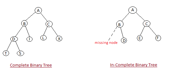
- Shape Property : Heap data structure is always a Complete Binary Tree, which means all levels of the tree are fully filled.
- Heap Property : All nodes are either [greater than or equal to] or [less than or equal to] each of its children. If the parent nodes are greater than their children, heap is called a Max-Heap, and if the parent nodes are smalled than their child nodes, heap is called Min-Heap.

How Heap Sort Works
Initially on receiving an unsorted list, the first step in heap sort is to create a Heap data structure(Max-Heap or Min-Heap). Once heap is built, the first element of the Heap is either largest or smallest(depending upon Max-Heap or Min-Heap), so we put the first element of the heap in our array. Then we again make heap using the remaining elements, to again pick the first element of the heap and put it into the array. We keep on doing the same repeatedly untill we have the complete sorted list in our array.
In the below algorithm, initially heapsort() function is called, which calls buildheap() to build heap, which inturn uses satisfyheap() to build the heap.
Sorting using Heap Sort Algorithm
/*  Below program is written in C++ language  */

void heapsort(int[], int);
void buildheap(int [], int);
void satisfyheap(int [], int, int);

void main()
{
  int a[10], i, size;
  cout << "Enter size of list";    // less than 10, because max size of array is 10
  cin >> size;
  cout << "Enter" << size << "elements";
  for( i=0; i < size; i++)
  {
    cin >> a[i];
  }
  heapsort(a, size);
  getch();
}

void heapsort(int a[], int length)
{
  buildheap(a, length);
  int heapsize, i, temp;
  heapsize = length - 1;
  for( i=heapsize; i >= 0; i--)
  {
    temp = a[0];
    a[0] = a[heapsize];
    a[heapsize] = temp;
    heapsize--;
    satisfyheap(a, 0, heapsize);
  }
  for( i=0; i < length; i++)
  {
    cout << "\t" << a[i];
  }
}

void buildheap(int a[], int length)
{
  int i, heapsize;
  heapsize = length - 1;
  for( i=(length/2); i >= 0; i--)
  {
    satisfyheap(a, i, heapsize);
  }
}

void satisfyheap(int a[], int i, int heapsize)
{
  int l, r, largest, temp;
  l = 2*i;
  r = 2*i + 1;
  if(l <= heapsize && a[l] > a[i])
  {
    largest = l;
  }
  else
  {
    largest = i;
  }
  if( r <= heapsize && a[r] > a[largest])
  {
    largest = r;
  }
  if(largest != i)
  {
    temp = a[i];
    a[i] = a[largest];
    a[largest] = temp;
    satisfyheap(a, largest, heapsize);
  }
}
Complexity Analysis of Heap Sort
Worst Case Time Complexity : O(n log n)
Best Case Time Complexity : O(n log n)
Average Time Complexity : O(n log n)
Space Complexity : O(n)
- Heap sort is not a Stable sort, and requires a constant space for sorting a list.
- Heap Sort is very fast and is widely used for sorting.
Searching Algorithms on Array
Before studying searching algorithms on array we should know what is an algorithm?
An algorithm is a step-by-step procedure or method for solving a problem by a computer in a given number of steps. The steps of an algorithm may include repetition depending upon the problem for which the algorithm is being developed. The algorithm is written in human readable and understandable form. To search an element in a given array, it can be done in two ways Linear search and Binary search.
Linear Search
A linear search is the basic and simple search algorithm. A linear search searches an element or value from an array till the desired element or value is not found and it searches in a sequence order. It compares the element with all the other elements given in the list and if the element is matched it returns the value index else it return -1. Linear Search is applied on the unsorted or unordered list when there are fewer elements in a list.
Example with Implementation
To search the element 5 it will go step by step in a sequence order.

function findIndex(values, target)
 {
   for(var i = 0; i < values.length; ++i)
     {
       if (values[i] == target)
         {
           return i;
         }
     }
   return -1;
 }
//call the function findIndex with array and number to be searched
findIndex([ 8 , 2 , 6 , 3 , 5 ] , 5) ;
Binary Search
Binary Search is applied on the sorted array or list. In binary search, we first compare the value with the elements in the middle position of the array. If the value is matched, then we return the value. If the value is less than the middle element, then it must lie in the lower half of the array and if it’s greater than the element then it must lie in the upper half of the array. We repeat this procedure on the lower (or upper) half of the array. Binary Search is useful when there are large numbers of elements in an array.
Example with Implementation
To search an element 13 from the sorted array or list.

function findIndex(values, target)
{
  return binarySearch(values, target, 0, values.length - 1);
};

function binarySearch(values, target, start, end) {
  if (start > end) { return -1; } //does not exist

  var middle = Math.floor((start + end) / 2);
  var value = values[middle];

  if (value > target) { return binarySearch(values, target, start, middle-1); }
  if (value < target) { return binarySearch(values, target, middle+1, end); }
  return middle; //found!
}

findIndex([2, 4, 7, 9, 13, 15], 13);
In the above program logic, we are first comparing the middle number of the list, with the target, if it matches we return. If it doesn’t, we see whether the middle number is greater than or smaller than the target.
If the Middle number is greater than the Target, we start the binary search again, but this time on the left half of the list, that is from the start of the list to the middle, not beyond that.
If the Middle number is smaller than the Target, we start the binary search again, but on the right half of the list, that is from the middle of the list to the end of the list.
